Opinion mining (sometimes known as sentiment analysis or emotion AI) refers to the use of natural language processing, text analysis, computational linguistics, and biometrics to systematically identify, extract, quantify, and study affective states and subjective information. Sentiment analysis is widely applied to the voice of the customer materials such as reviews and survey responses, online and social media, and healthcare materials for applications that range from marketing to customer service to clinical medicine. Industrial circles utilize opinion mining techniques to detect people’s preference for further recommendations, such as movie reviews and restaurant reviews. Thus, in this project, we are going to use a convolutional network (CNN) to perform sentiment sentence classification on the Stanford Sentiment Treebank (SST) dataset.

Stanford Sentiment Treebank

SST dataset has been initially introduced by Stanford to evaluate the performance of the, at that time novel, Recursive Neural Tensor Networks. It has been created extracting 11855 sentences from the movie reviews website Rotten Tomatoes and labeled into 5 categories, from 0 to 4 expressing different levels of satisfaction: very negative, negative, neutral, positive, and very positive respectively. It also exists a binary version (negative or positive) of the dataset but for this purpose, we won’t take this version into consideration. Moreover, the dataset presents a particular binary tree structure where the full sentence is the root, intermediate phrases correspond to the internal nodes and single words lay at the leaves.

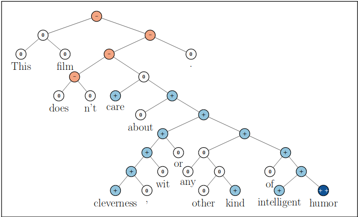
This structure permits to easily label not only the root (whole sentence) but also each phrase and word in the tree, hence taking advantage of them to further improve classification results using a kind of recursive model. Anyway, for this scope, we ignore the tree structure and each tree has been parsed such to have the typical label-sentence structure where the label corresponds to the label of the root.

Following, there are some sample sentences taken from the dataset with their corresponding label annotated on the right.

• 4 – a stirring, funny and finally transporting re-imagining of beauty and the beast and 1930s horror films.
• 3 – this is a visually stunning rumination on love, memory, history, and the war between art and commerce.
• 2 – you end up simply admiring this bit or that, this performance or that.
• 1 – apparently reassembled from the cutting-room floor of any given daytime soap.
• 0 – an ugly-duckling tale so hideously and clumsily told it feels accidental.

Convolutional Sentiment Analysis

Traditionally, CNNs are used to analyze and classify images sliding one or more convolutional filters (also known as kernels or receptive fields) grouped in a convolutional layer, sometimes followed by a max pooling layer to extract the most useful information from the resulting feature maps. After going through a set of convolutional layers, the final feature maps are usually flattened and used to feed a dense network to perform the final classification. The intuitive idea behind the learning process is that the network’s convolutional layers behave like feature extractors, hence hierarchically extracting parts of the image that are most useful to perform the classification.

Nevertheless, convolutional networks are also suitable for text classification tasks if we consider a sentence like a particular image. Specifically, a 2D image has three dimensions: height, width, and channels (usually 3 in the case of RGB images). Similarly, in the natural language processing field, we can consider a sentence like an image whose height corresponds to the length l of the sentence, its width corresponds to the embedding size d of its words and the number of channels is fixed to 1. Thus, in the same way, a 3 x 3 filter can look over a patch of an image, a 2 x d filter can look over 2 sequential words in a piece of text (bi-gram), 3 x d filters can look over tri-grams and n x d filters can search for useful n-grams.

As we can see in the above figure, each convolution on a set of n consecutive words (2 in the above example), will result in single output value. Thus, after the filter would have convolved over the whole sentence, we obtain an array of l – n +1 values (in the example l=4 and n=2, thus we obtain an array of 3 values), that is a feature map. Anyway, we have to take into account the fact that a convolutional layer has usually many filters, not just one, and each filter will learn to extract different features from the given image or text. Hence, the output of a filter consists of f feature maps where f is the number of filters. Next, each of its output feature maps is passed through a max-pooling layer which will select the maximum value of each map that corresponds to the n-gram the filter retains to be the most useful.

In this way, we would obtain an array v_n of f values where each value corresponds to the most useful n-gram extracted by each filter. Nevertheless, one convolutional layer, having a set of filters of the same size, is able to search only for some fixed size n-grams. Thus, a network consists of many convolutional layers c₂, …, c_n where each layer learns to look for its own n-grams (c₂ will learn to find interesting bi-grams, c₃ for tri-grams and so on).

The next layer is a concatenation layer, it will basically concatenate all the arrays v₂, v₃, … v_n obtained by the convolutional layers in a new array v whose length h is equal to the number of convolutional layers times the number of filters in each layer f (which is the same for each layer).

The intuition here is that we will be looking for the presence of different n-grams that are relevant for understanding the sentiment of a sentence.

On top of the concatenation layer lies a dense network used for classification. This dense network can have zero or more hidden layers of size h and an output dense layer with output size 5 to perform the final classification.

Data preprocessing

Before training the model, as common in NLP tasks, the row input sentences have been preprocessed in order to make them more easily understandable for the CNN model. In particular, it has been applied the following text preprocessing pipeline:

• Removal of punctuation;
• Characters lower case conversion;
• Filtering of non-purely alphabetical words;
• Filtering of stop words;
• Filtering of words less than two characters long;
• Filtering of words appearing in total less than two times in the training set;
• Sentence truncation to 50 words long (shorter sentences have been zero-padded).

Furthermore, the dataset has also been divided into train, validation, and test set.

Results

For all the experiments has been used a batch size of 32, Adam as optimizer, cross entropy as loss function and has been adopted early stopping to choose the model achieving the lowest validation loss to perform evaluation on the test set at the end of the 20 epochs of training. When dropout has been applied, it has been used the same dropout on both embedding and dense layers. In table 1, when embedding is None, it means that it hasn’t been used any pretrained embedding, hence the model learned a new embedding from scratch with an embedding size 300. On the other way, Glove300 means that the model’s embedding layer has been initialized with Glove embedding trained on 6 billions tokens and an embedding size of 300. Regarding the convolutional layers, the column Filters specifies the number of layers along with their filter size (i.e “2,3,4” means the network has 3 layers with a filter size of 2, 3 and 4 respectively). Moreover, each filter has a fixed number of output channels of 100. Have also been tried other values such as 20, 50 and 150 but the result were similar to the 100 version so they haven’t been reported on the result table. Finally, the parameter Hiddens specifies the number of hidden of the dense network (0 means that there is only the output layer).

Analyzing the results obtained in table 1, in the first row we have a simple model without dropout or pretrained embedding. We can clearly see that it strongly overfits the training data since the loss on the training set is 0.034 and the loss on the validation set is 1.661.

Hence, in the second experiment has been used a dropout of 0.2 and has been observed its effectiveness. Adding dropout the loss on the training set increased to 0.481 but the loss on the validation set decreased down to 1.609. The model still presents a problem of overfitting but less marked compared to the vanilla version without dropout. In the third experiment have been tested different numbers of convolutional layers and filter sizes. After testing different combinations, it emerged that combinations of 4 layers with filter sizes of 1,2,3 and 5 resulted in the best performance, thus further reducing the loss on the validation set down to 1.507.

Nevertheless, the three above mentioned models still achieve similar performance on the test set with an accuracy of around 30%. Thus, to further improve the model, it has been used a pretrained Glove embedding and has been observed that its addition significantly boosted the model performance. In particular, the loss on the training set increased to 0.623 and the loss on the validation set decreased to 1.477, thus further reducing overfitting. Moreover, the model achieved a 0.36% accuracy on the test set which is by far better than the accuracy obtained by the previous three models.

Finally, it has been placed a hidden layer right before the dense output layer. This addition gave another huge benefit to the final performance of the model lowering the loss on the validation set to 1.371 and achieving a 0.41% accuracy on the test set which is the best results this model achieved.

Conclusions

Despite the improvements obtained by fine-tuning the hyper-parameters of the convolutional model, vanilla convolution layers still suffer the problem of lack of recurrence, In fact, the result of the convolution on one n-gram is not influenced by the convolution on the n-gram before. For this purpose, convolutional layers with recurrent neural filters (RNF) have been proposed in 2018 and achieved an accuracy score of 53.4%. Anyway, pretrained models such as Elmo and Bert further improves the results on this dataset with the last one obtaining a good 55.5% accuracy on the test set in 2019.

Find more on

• https://github.com/davide97l/Sentiment-analysis

References

• https://github.com/bentrevett/pytorch-sentiment-analysis
• https://nlp.stanford.edu/sentiment/treebank.html
• https://paperswithcode.com/sota/sentiment-analysis-on-sst-5-fine-grained